
Section navigation is enabled for this long article; the full text remains continuous.
Why can the same factor have different associations with health in different places and periods? This question motivates BSTVC, our Bayesian spatiotemporally varying coefficients framework.
BSTVC Desktop brings the framework into a graphical research environment. Researchers can prepare geographic data, check its alignment with a map, fit a suitable model, and export results for interpretation. These six cases show the workflow across continuous outcomes, binary outcomes, counts, and a spatial cross-section.
The full-size figures below come from the supplied English illustrated user guide for BSTVC Desktop 26.08.01. The result plots use its companion R visualization workflow after exporting model tables. They are tutorial outputs; no models were rerun for this article.

From data to interpretable results
Start with a table and a geographic map. Each panel row represents one place at one time; a spatial cross-section has one row per place.
- Reshape wide, time-labelled tables with Data Conversion when needed.
- Load the table and map components in Data Input.
- Run Data Check to verify identifiers and observation order.
- Choose BSTVC for a space-time panel or BSVC for a spatial cross-section, with a response family appropriate to the outcome.
- Inspect diagnostics, export the results, and visualize estimates with uncertainty.
Interpretability is built into the estimated model parameters. Spatial and temporal coefficients describe local variation. The spatiotemporal variance partitioning index (STVPI) summarizes contributions within the model. Fitted values and prediction outputs describe the outcome. Together, these views connect local patterns with a broader assessment of the research question.
Case 1. Under-five mortality across Africa
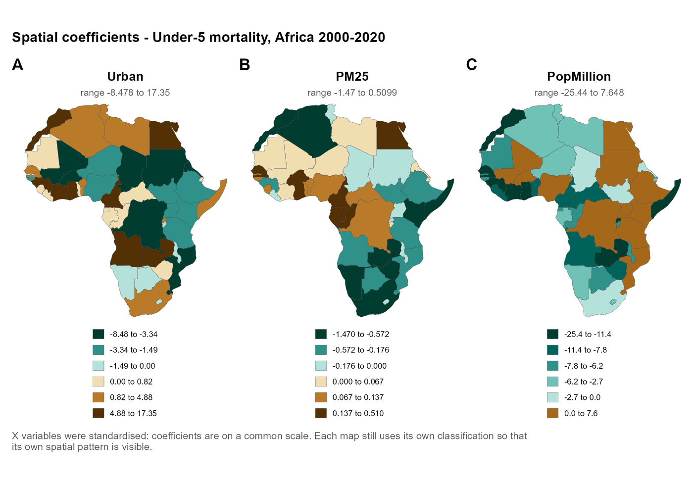
This continuous-outcome example follows 48 African countries over 2000–2020: 1,008 country-years. Under-five mortality is measured as deaths per 1,000 live births. The illustrated run includes urban population share, PM2.5 exposure, and population size.
The coefficient maps show why geographic variation matters. The estimated urbanization association takes both positive and negative values across countries, a pattern concealed by a single overall coefficient. Each panel has its own legend, so matching colors across panels does not imply matching values. These are estimated associations; uncertainty and study context remain part of their interpretation.
Case 2. Monthly COVID-19 outbreak status in China
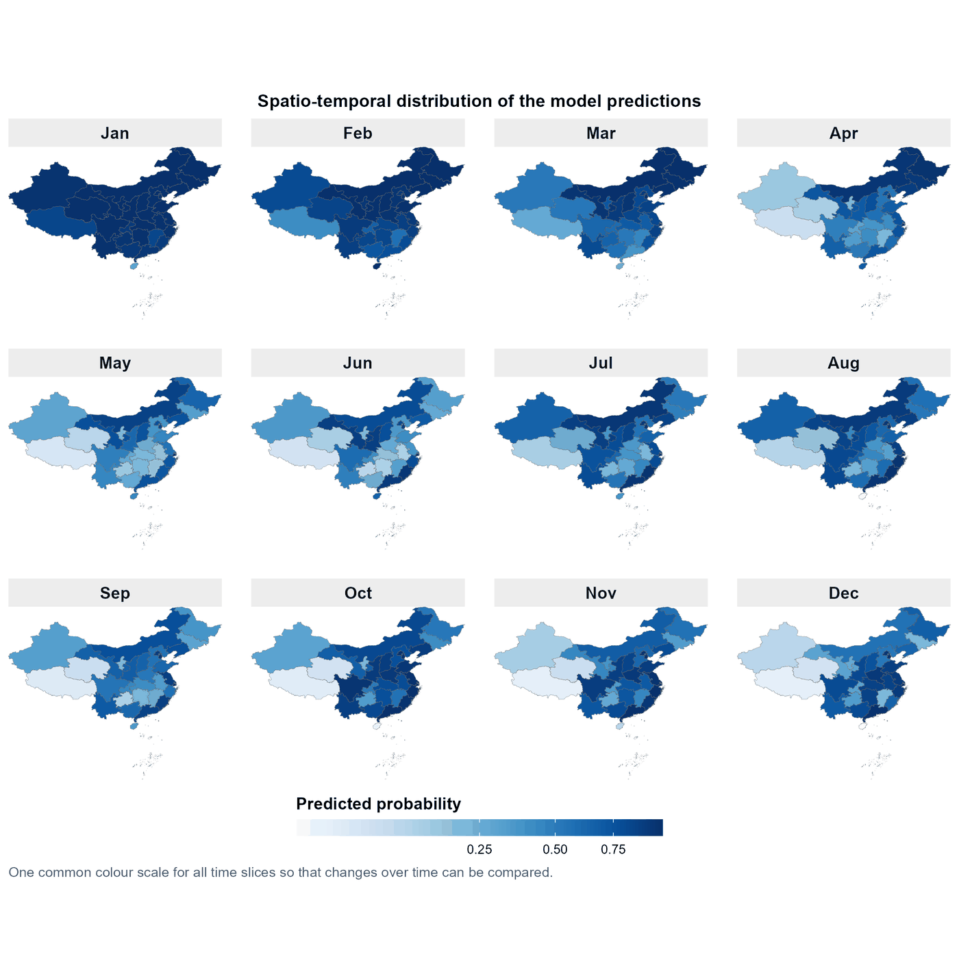
The starting table covers 31 mainland-China provincial units during the twelve months of 2020. Data Conversion reshapes its time-labelled columns into 372 province-month records.
A binary model then relates outbreak status to environmental indicators and migration indices. Its fitted output is a probability, rather than a case count. All twelve maps share one probability scale, making the monthly historical pattern easier to compare. The example demonstrates wide-to-panel conversion and binary modeling; forecasting future outbreaks would require separate validation.
Case 3. Acute hepatitis B counts in five US states
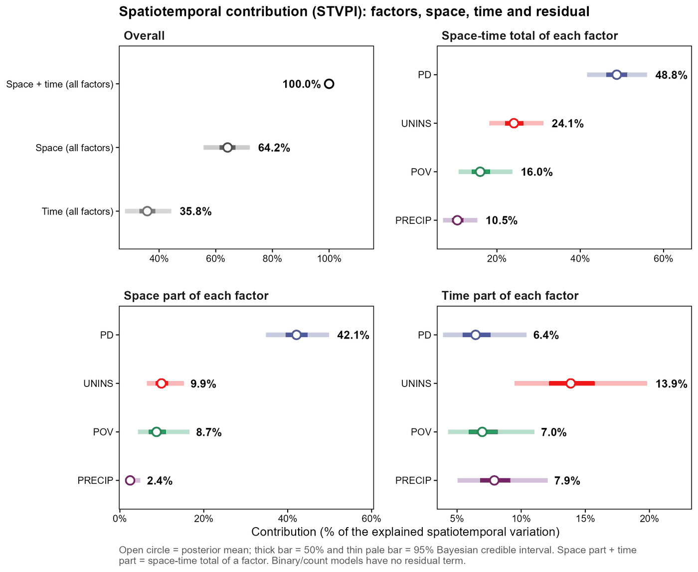
This count/Poisson example covers Kentucky, North Carolina, Tennessee, Virginia, and West Virginia during 2012–2023. The converted table has 60 state-year records. The outcome is the number of acute hepatitis B surveillance cases, with population density, uninsured rate, poverty, and precipitation as candidate variables.
The STVPI plot displays posterior means with 50% and 95% credible intervals. It offers a useful way to read estimated contributions alongside uncertainty. With only five areas, the case is primarily a workflow demonstration. In this guide's count run, percentages are relative among included covariates, with no residual component; 100% does not mean that all disease variation has been explained.
Case 4. One US panel, two outcome definitions
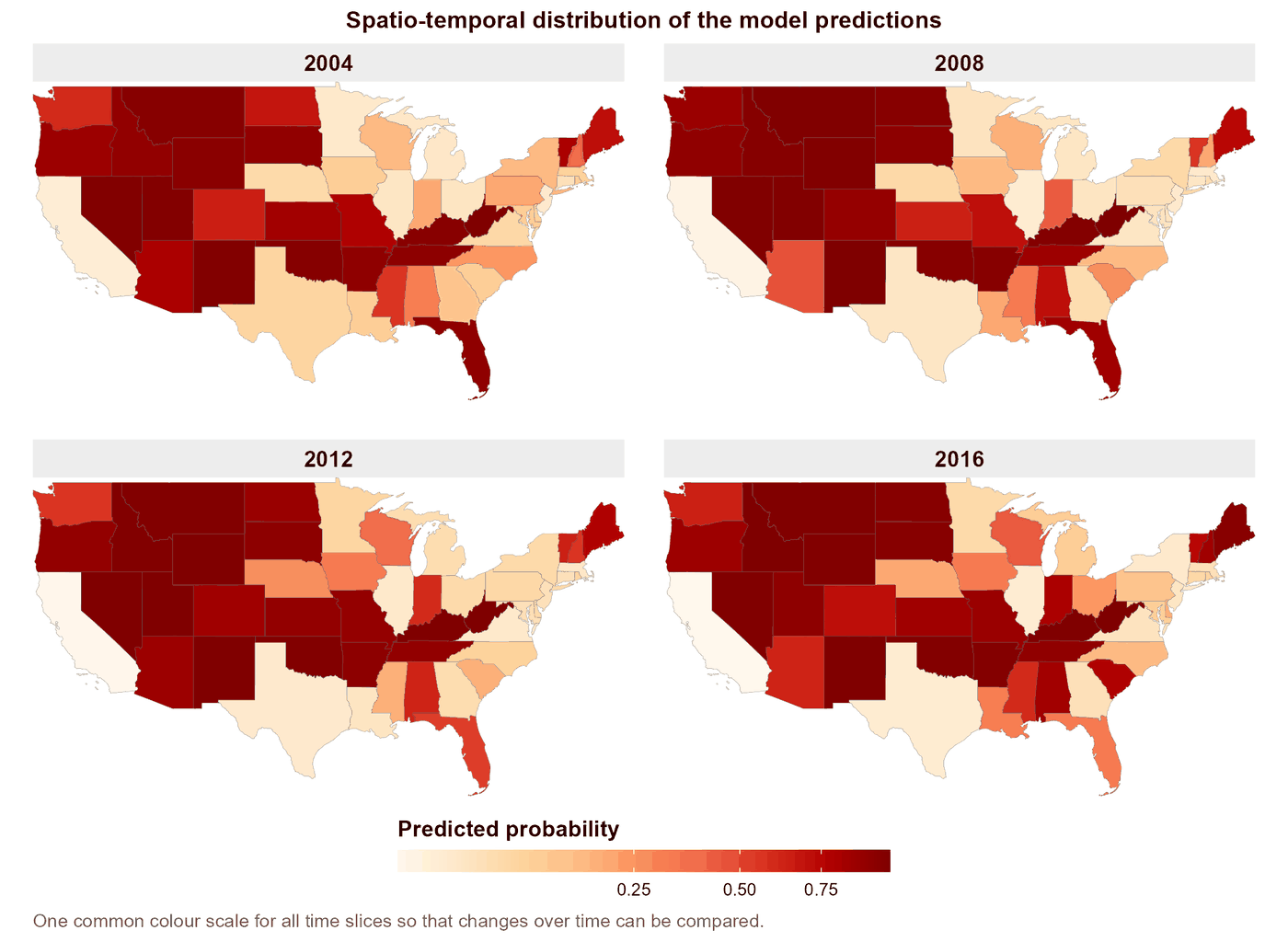
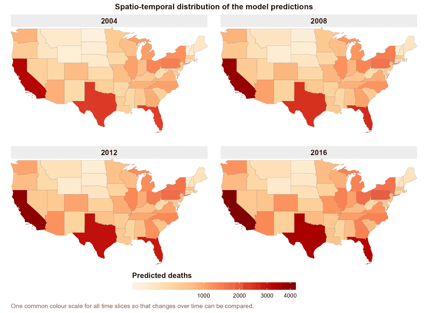
The fourth case contains 637 observations: 49 US areas, comprising the contiguous states and the District of Columbia, over 2004–2016.
The binary analysis asks whether an area's age-adjusted suicide rate exceeds the median across those areas in the same year. This is a derived teaching indicator. The count analysis models recorded deaths. The two maps therefore answer different questions and use different scales.
The guide also documents a numerical problem with standardized predictors in its count run and healthier diagnostics with unstandardized predictors. This dataset-specific lesson reinforces the value of checking evaluation tables before interpreting results. The count run's nearly uniform contribution shares do not support a useful factor ranking. These analyses describe aggregate areas, not individual risk.
Case 5. A spatial-only analysis for 2016
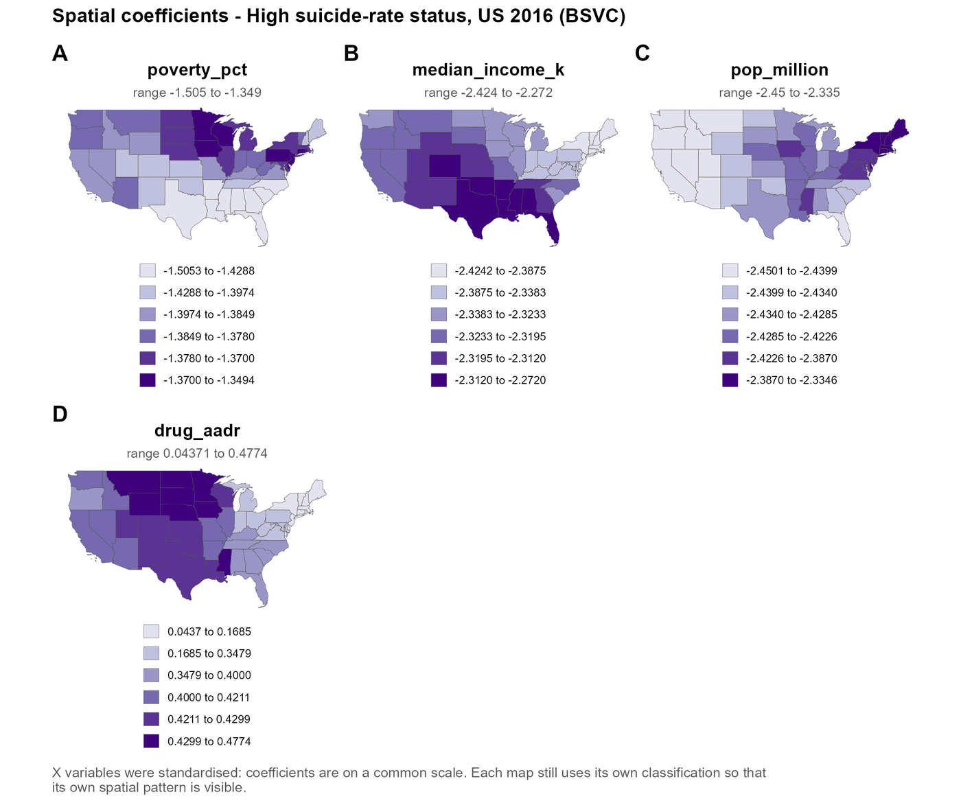
Keeping only the 2016 observations from Case 4 gives one record for each of the 49 areas. This calls for the BSVC module and the spatial cross-section Data Check mode.
The outcome remains the derived above-median area-rate indicator. The four maps show spatial coefficient estimates for the included variables. There is no time field or temporal coefficient output: a one-year dataset cannot establish change over time. The guide also reports wide contribution intervals, so the example is better suited to learning the spatial-only workflow than confidently ranking factors.
Case 6. Global health-adjusted life expectancy
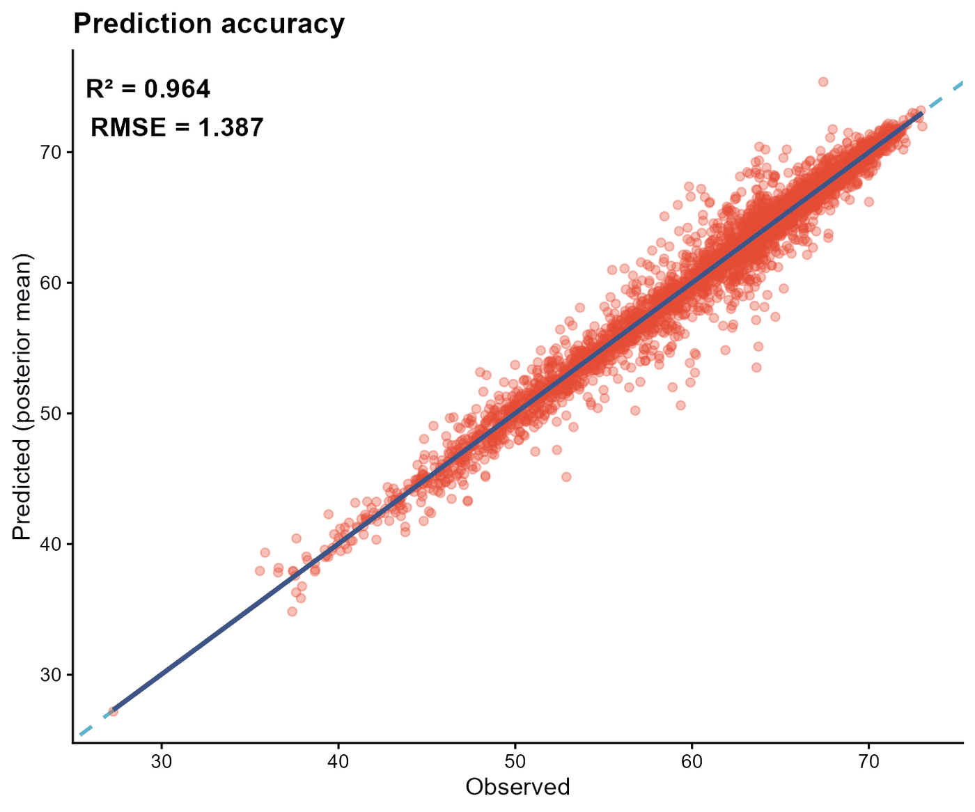
The final case models health-adjusted life expectancy (HALE), in years, across 177 countries and regions over 2000–2020. The full panel contains 3,717 country-year cells. The English-guide run uses twelve explanatory variables, with 3,444 observed outcome values in the displayed fit comparison.
The observed-versus-fitted plot reports R-squared of about 0.96 and RMSE of about 1.39 years. These are in-sample reference results: the guide fits and evaluates on the same data without a hold-out set. The close fit is informative for model checking; performance on new places or future years needs independent assessment.
What to take into your own analysis
Choose an outcome and response family that match your question. Verify map identifiers and observation order before fitting. Read evaluation tables, coefficient uncertainty, and contribution estimates together. Preserve legends and axes when sharing figures, and separate fitted performance from validation on new data.
BSTVC Desktop makes the modeling sequence more accessible. Data quality, sensitivity analysis, and domain knowledge remain essential. These area-level tutorial associations do not establish causal effects.
Download, documentation, and the team
BSTVC Desktop is developed within the HEOA–West China Health & Medical Geography Group. Chao Song leads the project and statistical methodology; Xianteng Tang develops the software and supports its use.
The software is free for academic and other noncommercial use under the project's PolyForm Noncommercial License 1.0.0. Commercial use requires a separate license; consult the linked terms.
- BSTVC Desktop official website
- English Windows release v2026.8.1 and installer
- English online user guide
- Chinese desktop website and documentation
- BSTVC research ecosystem
- BSTVC-R for scripted workflows
- Software license
Start with the example closest to your outcome and data structure. Follow the checks, inspect the exported tables, and then adapt the workflow to your own research question.
Figure source: BSTVC Desktop English Illustrated User Guide V03, supplied in 1_Guide.rar. Case descriptions follow the English source; the Chinese guide provided a terminology cross-check. The public online guide is a separate resource and may present different examples.