Can Every Place Have Its Own Time Trend?

BSTVC & Spatiotemporal Interpretability · Part 4 Chao Song · 27 October 2026

A coefficient map can vary across places. A coefficient curve can vary across years. Put them together, and every place can have a time-varying coefficient—but not necessarily its own pattern of change.

The useful distinction: a shared temporal change is different from a place-specific temporal change. Before interpreting a colourful space–time display, check which one the model can represent.

A map plus a curve

In the original STVC formulation, spatial and temporal coefficient components enter additively. The 2024 hospital-bed application makes this especially clear in Equation 4: a covariate is multiplied by a spatial coefficient and by a temporal coefficient, and those contributions are added. [1, 2]

For one covariate, suppress its index and write the combined coefficient as:

b(i,t) = μ(i) + γ(t)

Here μ(i) is the place component and γ(t) is the time component. This simplified expression isolates the coefficient; it is not the full likelihood, intercept structure or estimation specification.

Two consequences follow directly from the arithmetic:

• Between places A and B at the same time: b(A,t) − b(B,t) = μ(A) − μ(B). The coefficient gap stays constant.
• Between times 1 and 2 at the same place: b(i,2) − b(i,1) = γ(2) − γ(1). Every place shares that temporal change.

The curve need not be a straight line. It can rise, fall or bend. Under this additive structure, however, all places inherit the same changes, shifted up or down by their spatial components.

See the restriction

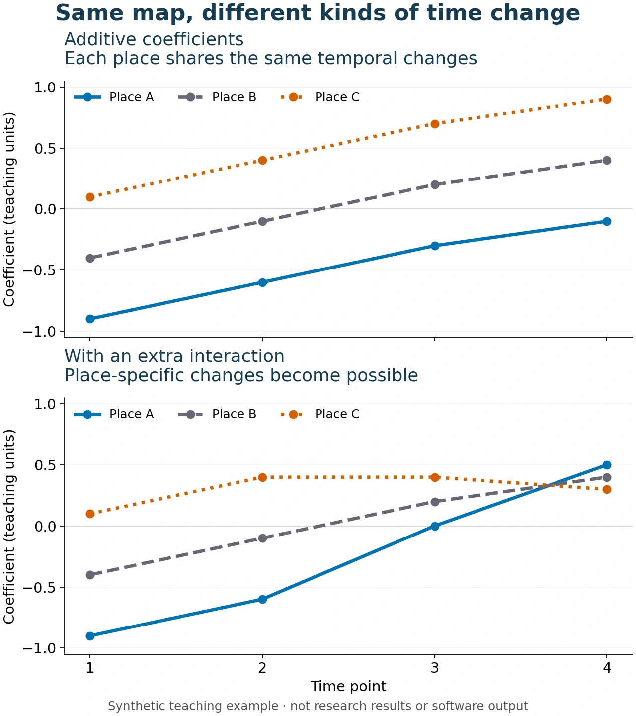
Figure 1. Synthetic teaching example, not fitted results or BSTVC Desktop output. Top: μ = (−0.5, 0, 0.5) and γ = (−0.4, −0.1, 0.2, 0.4). Bottom: add an illustrative place–time component of (0, 0, 0.3, 0.6) for A, zeros for B, and (0, 0, −0.3, −0.6) for C. Values are arbitrary teaching units, not estimated parameters or a fully constrained model.

In the upper panel, A moves from −0.9 to −0.1 and C from 0.1 to 0.9. Their gap remains 1.0. All three places change by 0.3, then 0.3, then 0.2.

In the lower panel, A and C no longer share those increments. Writing b(i,t) = μ(i) + γ(t) + δ(i,t) can represent that additional structure. A non-additive δ allows changes that a place effect plus a common time effect cannot reproduce. This is a conceptual comparison—not a claim that a particular software release implements this interaction.

Three interpretation traps

Coefficient trends are not outcome trends. Even with additive coefficients, observed outcomes and fitted means can follow different trajectories across places: covariates, other model terms and the link function also matter. The restriction above applies to the coefficient on its specified scale.

A decomposition needs identification. Moving a constant from μ to γ leaves their sum unchanged. Actual models need appropriate constraints or parameterisation. Our teaching numbers illustrate the sum; they are not a complete fitting recipe.

Two uncertainty bands cannot simply be added. Uncertainty for μ + γ depends on their joint posterior, including covariance. Combining marginal interval endpoints does not generally produce a valid credible interval for the sum.

What to check before your next analysis

Ask one precise question: Do I need different coefficient levels across places, or different temporal changes across places? Read the actual model equation and versioned documentation before choosing a specification. More flexibility is not automatically better; it needs enough information, defensible priors and validation matched to the intended use.

This distinction supports the BSTVC team's work on Spatiotemporal Interpretability: make clear what varies, on which scale, and under which assumptions. These are conditional associations, not causal effects.

Start with the BSTVC organisation website and BSTVC Desktop documentation and downloads. Free use is limited to academic and non-commercial purposes; consult the current official licence for exact terms.

中文速读

空间系数加时间系数，允许地区水平不同、共同时间曲线变化，却不等于每个地区都有独立的变化轨迹。这里的限制针对系数，而不是观测结局。需要地区特有的时间变化时，应核对是否明确建模了时空交互，并检查识别约束、不确定性与验证；更复杂不代表更好。图中均为教学设定，不是软件运行或真实研究结果。

Sources and series

1. Song, C., Shi, X. & Wang, J. (2020). Spatiotemporally Varying Coefficients (STVC) model: a Bayesian local regression to detect spatial and temporal nonstationarity in variables relationships. Annals of GIS, 26(3), 277–291. Original article, Equation 2. Author-uploaded full text inspected for the additive specification.
2. Song, C., Fang, L., Xie, M., et al. (2024). Revealing spatiotemporal inequalities, hotspots, and determinants in healthcare resource distribution: insights from hospital beds panel data in 2308 Chinese counties. BMC Public Health, 24, 423. Open-access full text, Equation 4.

The algebra and numerical figure are original teaching derivations from the stated additive form. Sources checked 27 October 2026. No model was fitted for this article.

Previous: Similar neighbours, different relationships · Series introduction · BSTVC research hub