Reading a Coefficient Map Without Losing Its Uncertainty

BSTVC & Spatiotemporal Interpretability · Part 5

Chao Song · 28 October 2026

Three regions can have the same colour on a coefficient map—and very different evidence about the direction of an association. A map of posterior means shows one summary per place. It does not show how widely the posterior distribution spreads around that summary.

The practical rule: read the estimate, its uncertainty and its meaning together.

First, identify what is mapped

The 2020 STVC methods paper estimates spatial and temporal coefficient components within a Bayesian hierarchical model, with uncertainty represented in the posterior. A coefficient describes a conditional association, not automatically a causal effect. Read the 2020 methods paper.

Before interpreting colour, check the covariate's units, transformations and coefficient scale. Also check whether the map shows a spatial component or a combined coefficient. As Part 4 explains, adding spatial and temporal components requires carrying their joint uncertainty—not simply adding interval endpoints.

What a 95% credible interval says

An equal-tailed 95% credible interval runs from the posterior's 2.5th percentile to its 97.5th percentile. Under the specified model and observed data, it contains 95% of the posterior probability for that parameter. Numerical inference may approximate this distribution. This is uncertainty about the coefficient, not a prediction interval for future observations.

That statement is conditional on the likelihood, priors, covariates and dependence structure. It does not guarantee that these choices are correct, cover every source of bias, or assign 95% probability to the whole map being correct. Individual intervals are not a simultaneous uncertainty region for every mapped coefficient.

INLA's official documentation distinguishes posterior summaries from posterior marginal distributions and provides quantile and distribution functions for those marginals. Posterior outputs · Marginal functions.

Same mean, different certainty

Consider three synthetic teaching distributions, all with mean 0.30, but with normal posterior standard deviations of 0.10, 0.25 and 0.40. These are assumed distributions in arbitrary coefficient units, not fitted BSTVC results or software output. Real posterior marginals need not be normal.

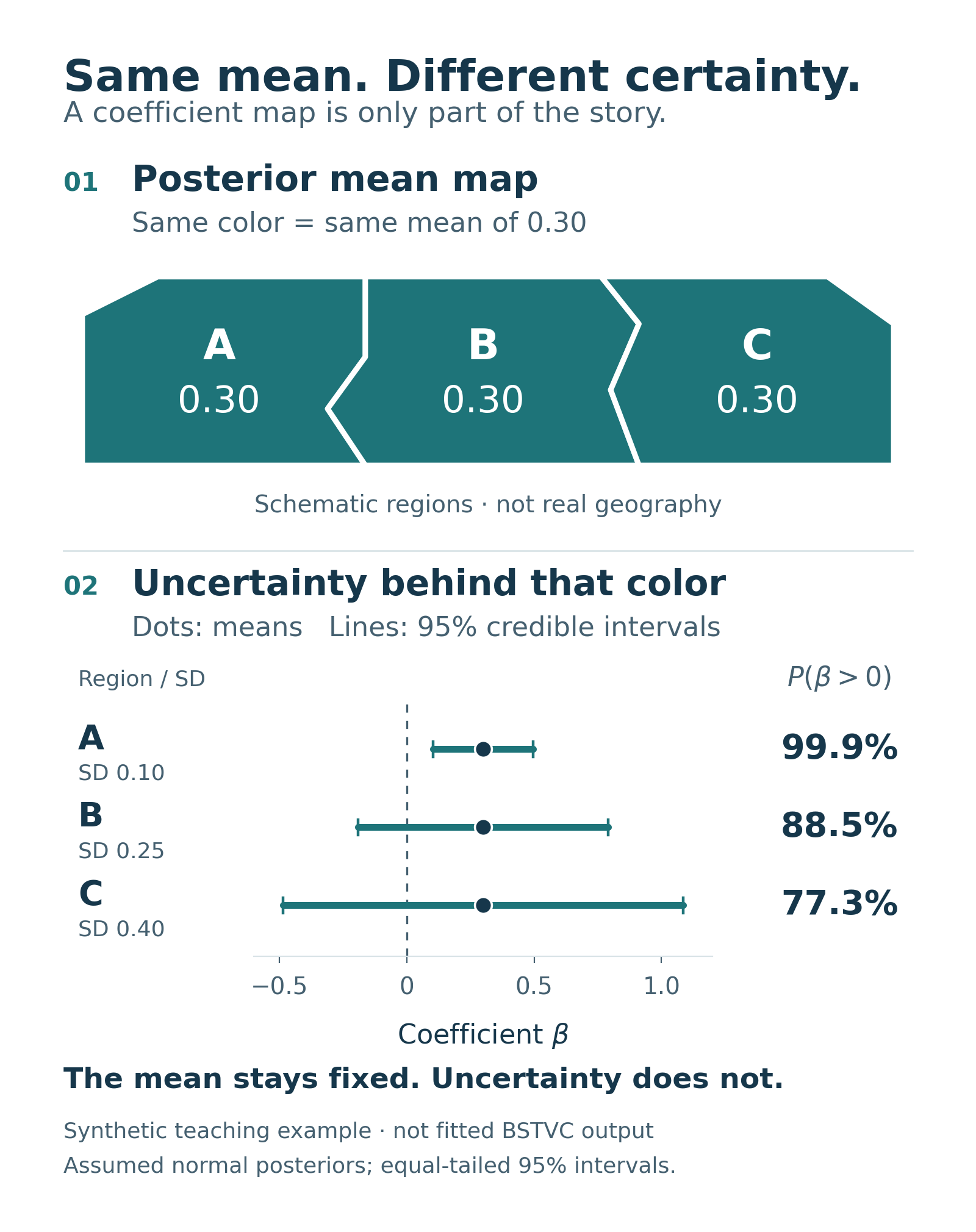
Figure 1. Same mean, different certainty. Original synthetic teaching example, not real geography or fitted BSTVC output. Each interval contains 95% of its assumed normal posterior. The values below are readable as text; the sign probabilities are model-conditional, not causal probabilities.

• A: mean 0.30; 95% interval 0.104 to 0.496; probability above zero 99.9%.
• B: mean 0.30; 95% interval −0.190 to 0.790; probability above zero 88.5%.
• C: mean 0.30; 95% interval −0.484 to 1.084; probability above zero 77.3%.

A mean-only map gives all three regions the same colour. Their uncertainty tells a different story: A's distribution is tightly concentrated above zero; B and C leave more posterior probability on negative values.

An interval crossing zero does not establish “no association.” Nor does an interval excluding zero establish practical importance. Meaningful magnitude depends on the research question and measurement scale.

Read sign uncertainty directly

For a continuous coefficient, the posterior probability of a positive association is one minus its posterior cumulative probability at zero. INLA documents inla.pmarginal() for that cumulative probability; inla.qmarginal() supplies interval endpoints. These answer different questions: direction probability versus a range of plausible magnitudes. Official marginal documentation.

Neither quantity is a causal probability or a frequentist p-value. Report the actual probability or interval rather than reducing every region to a yes/no label.

Compare regions with a contrast

“Is A larger than B?” concerns the posterior of the difference, not whether two separate intervals overlap. That difference depends on their joint posterior, including covariance. INLA's official FAQ explains why a linear combination's uncertainty cannot be reconstructed from the separate marginals alone. Linear combinations in INLA.

For your next coefficient map, retain three companions: the estimand and scale, an uncertainty display, and a sentence stating the model-conditional interpretation. Check sensitivity and model adequacy before making substantive claims.

This article forms part of the BSTVC team’s work on Spatiotemporal Interpretability at the HEOA–West China Health & Medical Geography Group.

Explore the BSTVC organisation website and BSTVC Desktop documentation and downloads. BSTVC Desktop is available for academic and noncommercial use under its current PolyForm Noncommercial licence; commercial use requires separate permission. Consult the official licence for the exact terms applicable to your version and workflow.

中文速读

地图颜色通常只展示后验均值，不能代替不确定性。相同均值可能对应不同的95%可信区间和正向关联概率；可信区间跨零不等于“没有关联”，不跨零也不等于影响重要或存在因果关系。可信区间以数据和模型设定为条件。比较地区时，应分析系数差的联合后验，而不是把区间是否重叠当作检验。图表中的三个地区均为教学设定，不是真实研究或软件运行结果。

Sources and series

• Song, C., Shi, X. & Wang, J. (2020). Spatiotemporally Varying Coefficients (STVC) model: a Bayesian local regression to detect spatial and temporal nonstationarity in variables relationships. Annals of GIS, 26(3), 277–291. Original article · Author-uploaded full text.
• R-INLA: model outputs, marginal functions, and linear-combination FAQ.
• Krainski, E. T. & Rue, H. A short introduction on how to fit a SPDE model with INLA, §5.1 (last updated 2017). Official worked-example PDF.
• Sources checked 28 October 2026. The normal distributions and calculations above are an original teaching example; no model was fitted.

Previous: Can Every Place Have Its Own Time Trend?